RL_Paper_03:Rainbow

Rainbow: Combining Improvements in Deep Reinforcement Learning

Paper Source
Journal: AAAI
Year: 2017
Institute: DeepMind
Author: Matteo Hessel, Joseph Modayil, Hado van Hasselt
#Deep Reinforcement Learning

Abstract

This paper examines six main extensions to DQN algorithm and empirically studies their combination. (It is a good paper which gives you a summary of several important technologies to alleviate the problems remaining in DQN and provides you some valuable insights in this research region.)
Baseline: Deep Q-Network(DQN) Algorithm Implementation in CS234 Assignment 2

INTRODUCTION
Because the traditional tabular methods are not applicable in arbitrarily large state spaces, we turn to those approximate solution methods (linear approximator & nonlinear approximator value-function approximation & policy approximation), which is to find a good approximate solution using limited computational resources. We can use a linear function, or multi-layer artificial neural networks, or decision tree as a parameterized function to approximate the value-function or policy.(More, see Sutton’s book Reinforcement Learning: An Introduction Chapter 9).
The following methods are all value-function approximation and gradient-based(using the gradients to update the parameters), and they all use experience replay and target network to eliminate the correlations present in the sequence of observations.

1> Linear Function

Using a linear function to approximate the value function(always the action value).

$\hat v(s, w) \doteq w^Tx(s) \doteq \sum \limits_{i=1}^d w_i x_i$

$w$ is the parameters, $x(s)$ is called a feature vector representing state $s$, and the state $s$ is the images(frames) observed by the agent in most time. So a linear approximator implemented with tensorflow can be just a fully-connected layer.

import tensorflow as tf
# state: a sequence of image(frame)
inputs = tf.layers.flatten(state)
# scope, which is used to distinguish q_params and target_q_params
out = layers.fully_connected(inputs, num_actions, scope=scope, reuse=reuse)

2> Nonlinear - DQN

Deep Q-Network. The main difference of DQN from linear approximator is the architecture of getting the q_value, it is nonlinear.

And the total algorithm is as follows:

The approximator of DeepMind DQN implemented with tensorflow as described in their Nature paper can be:

import tensorflow as tf
with tf.variable_scope(scope, reuse=reuse) as _:
	conv1 = layers.conv2d(state, num_outputs=32, kernel_size=(8, 8), stride=4, activation_fn=tf.nn.relu)
	conv2 = layers.conv2d(conv1, num_outputs=64, kernel_size=(4, 4), stride=2, activation_fn=tf.nn.relu)
	conv3 = layers.conv2d(conv2, num_outputs=64, kernel_size=(3, 3), stride=1, activation_fn=tf.nn.relu)
	full_inputs = layers.flatten(conv3)
	full_layer = layers.fully_connected(full_inputs, num_outputs=512, activation_fn=tf.nn.relu)
	out = layers.fully_connected(full_layer, num_outputs=num_actions)

Do DQN from scratch(basic version)

3> Nonlinear - DDQN

Double DQN. The main difference of DDQN from DQN is the way of calculating the target q value.
As a reminder,
In Q-Learning:

$Q(s,a) \leftarrow Q(s,a) + \alpha[r + \lambda max_{a'}Q(s',a') − Q(s,a)]$ $Y_t^{Q} = R_{t+1} + \lambda max_{a'}Q(S_{t+1},a') = R_{t+1} + \lambda Q(S_{t+1},argmax_{a'}Q(S_{t+1},a'))$

In DQN:

where $\theta_{i-1}$ is the target network parameters which is always represeted with $\theta_t^-$.

$Y_t^{DQN} = R_{t+1} + \lambda max_{a'}Q(S_{t+1},a';\theta_t^-)$

There is a problem with deep q-learning that “It is known to sometimes learn unrealistically high action values because it includes a maximization step over estimated action values, which tends to prefer overestimated to underestimated values” as said in DDQN paper.
The idea of Double Q-learning is to reduce overestimations by decomposing the max operation in the target into action selection and action evaluation.

$Y_t^{DoubleQ} = R_{t+1} + \lambda Q(S_{t+1}, argmax_{a'}Q(S_{t+1},a';\theta_t);\theta_t^-)$

Implement with tensorflow (the minimal possible change to DQN in cs234 assignment 2)

# DQN
q_samp = tf.where(self.done_mask, self.r, self.r + self.config.gamma * tf.reduce_max(target_q, axis=1))
actions = tf.one_hot(self.a, num_actions)
q = tf.reduce_sum(tf.multiply(q, actions), axis=1)
self.loss = tf.reduce_mean(tf.squared_difference(q_samp, q))

# DDQN
max_q_idxes = tf.argmax(q, axis=1)
max_actions = tf.one_hot(max_q_idxes, num_actions)
q_samp = tf.where(self.done_mask, self.r, self.r + self.config.gamma * tf.reduce_sum(tf.multiply(target_q, max_actions), axis=1))
actions = tf.one_hot(self.a, num_actions)
q = tf.reduce_sum(tf.multiply(q, actions), axis=1)
self.loss = tf.reduce_mean(tf.squared_difference(q_samp, q))

Do Double DQN from scratch(basic version)

4>Prioritized experience replay

Prioritized experience replay. Improve data efficiency, by replaying more often transitions from which there is more to learn.
And the total algorithm is as follows:

Prioritizing with Temporal-Difference(TD) Error
TD-Error: how far the value is from its next-step bootstrap estimate $r + \lambda V(s') - V(s)$
Where the value $r + \lambda V(s’) $ is known as the TD target.
Experiences with high magnitude TD error also appear to be replayed more often. TD-errors have also been used as a prioritization mechanism for determining where to focus resources, for example when choosing where to explore or which features to select. However, the TD-error can be a poor estimate in some circumstances as well, e.g. when rewards are noisy.
Stochastic Prioritization
Because greedy prioritization results in high-error transitions are replayed too frequently causing lack of diversity which could lead to over-fitting. So Stochastic Prioritization is intruduced in order to add diversity and find a balance between greedy prioritization and random sampling.
We ensure that the probability of being sampled is monotonic in a transition’s priority, while guaranteeing a non-zero probability even for the lowest-priority transition. Concretely, the probability of sampling transition i as
$P(i) = \frac{p_i^{\alpha}}{\sum_kp_k^{\alpha}}$
(Note: the probability of sampling transition $P(i)$ has nothing to do with the probability to sample a transition(experience) in the replay buffer(sum tree), which is based on the transition’s priority $p_i$. So don’t be confused by it, the $P(i)$ is used to calculate the Importance Sampling(IS) Weight.)
where $p_i > 0$ is the priority of transition $i$. The exponent α determines how much prioritization is used, with $\alpha = 0$ corresponding to the uniform case.

proportional prioritization: $p_i = |\delta_i| + \epsilon$
rank-based prioritization: $p_i = \frac{1}{rank(i)}$ , where $rank(i)$ is the rank of transition $i$ sorted according to $\delta_i$.
Importance Sampling(IS)
Because prioritized replay introduces a bias that changes this distribution uncontrollably. This can be corrected by using importance-sampling (IS) weights:
$w_i = (\frac{1}{N} \frac{1}{P(i)})^\beta$
that fully compensate for the non-uniform probabilities $P(i)$ if $\beta = 1$. These weights can be folded into the Q-learning update by using $w_i\delta_i$ instead of $\delta_i$. For stability reasons, we always normalize weights by $1 / max_i w_i$ so that they only scale the update downwards.
IS is annealed from $\beta_0$ to $1$, which means its affect is felt more strongly at the end of the stochastic process; this is because the unbiased nature of the updates in RL is most important near convergence.

Do Double DQN with prioritized experience replay from scratch(basic version)

5>Dueling network architecture

Dueling network architecture. Generalize across actions by separately representing state values and action advantages.
The dueling network is a neural network architecture designed for value based RL which has a $|A|$ dimension output that Q-value for each action. It features two streams of computation, the state value and action advantage streams, sharing a convolutional encoder, and merged by a special aggregator layer.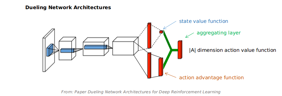

The aggregator can be expressed as:

$Q(s, a; \theta, \alpha, \beta) = V(s; \theta, \beta) + \big(A(s, a; \theta, \alpha) - \frac{1}{|A|} \sum_{a'}A(s, a'; \theta, \alpha)\big)$

where $\theta, \beta, \alpha$, respectively, the parameters of the shared convolutional encoder, value stream, and action advantage stream.
The details of dueling network architecture for Atari: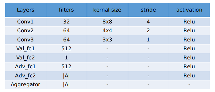

Since both the value and the advantage stream propagate gradients to the last convolutional layer in the backward pass, we rescale the combined gradient entering the last convolutional layer by $1/\sqrt{2}$. This simple heuristic mildly increases stability. In addition, we clip the gradients to have their norm less than or equal to $10$.

Other tricks:

Human Starts: Using 100 starting points sampled from a human expert’s trajectory.
Saliency maps: To better understand the roles of the value and the advantage streams.

Do Dueliing Double DQN with prioritized experience replay from scratch(basic version)

6>Multi-step bootstrapping

Multi-step bootstrap targets. Shift the bias-variance tradeoff and helps to propagate newly observed rewards faster to earlier visited states.
The best methods are often intermediate between the two extremes. n-step TD learning method lies between Monte Carlo and one-step TD methods.

Monte Carlo methods perform an update for each state based on the entire sequence of observed rewards from that state until the end of the episode
$G_t \doteq R_{t+1} + \gamma R_{t+2} + \gamma^2R_{t+3} + \dots + \gamma^{T−t−1}R_T$
The update of one-step TD methods(also called TD(0) methods), on the other hand, is based on just the one next reward, bootstrapping from the value of the state one step later as a proxy for the remaining rewards.
$G_{t:t+1} \doteq R_{t+1} + \gamma V_t(S_{t+1})$
Now, n-step TD methods perform a tradeoff that update each state after n time steps, based on n next rewards, bootstrapping from the value of the state n step later as a proxy for the remaining rewards.
$G_{t:t+n} \doteq R_{t+1} + \gamma R_{t+2} + \dots + \gamma ^{n−1}R_{t+n} + \gamma^n V_{t+n−1}(S_{t+n})$

We know that Q-learning is a kind of TD learning. All the implementations before are based on TD(0) learing updating. Now, we are going to implement a n-step deep Q-learning method, the most different part is how to calculate the target Q value.
In one-step DQN:

$q_{target} = R_{t+1} + \gamma_{t+1} \max q_{\bar{\theta}}(S_{t+1}, a')$

In one-step Double DQN, the loss is :

$q_{target} = R_{t+1} + \gamma_{t+1} q_{\bar{\theta}}(S_{t+1}, \arg\max_{a'} q_{\theta}(S_{t+1}, a'))$

In multi-step Double DQN, the loss is :

$R^{(n)}_t ≡ \sum\limits_{k=0}^{n-1} \gamma_t^{(k)}R_{t+k+1} \\ q_{target} = R^{(n)}_t + \gamma_{t}^n q_{\bar{\theta}}(S_{t+n}, \arg\max_{a'} q_{\theta}(S_{t+n}, a'))$

(The algorithm looks easy to implement and stability guaranteed, but it brings much fluctuation and seems learning rate sensitive when used to train the agent to play CartPole-v0. So if you check this model, you maybe should pay a little bit more attention to it.)
Do Multi-Step Dueliing Double DQN with prioritized experience replay from scratch(basic version)

7>Distributional Q-learning

Distributional Q-learning. Learn a categorical distribution of discounted returns, instead of its expectation.
In Q learning:

$Q(s, a) = \sum\limits_{i=0}^{n} p_{r_i}r_i(s, a) + \gamma \sum\limits_{s' \in S} P(s'|s, a)\max_{a' \in A(s')}Q(s', a') \\ = E_{s, a}[ r(s, a) ] + \gamma E_{s, a, s'}[ \max_{a' \in A(s')}Q(s', a') ] \\ = E_{s, a, s'}[ r(s, a) + \gamma \max_{a' \in A(s')}Q(s', a') ]$

Where $Q(s, a)$ is the expection of the discounted returns.
Now, in distributional rl, instead of calculating the expection, we work directly with the full distribution of the returns of state $s$, action $a$ and following the current policy $\pi$, denoted by a random variable $Z(s, a)$.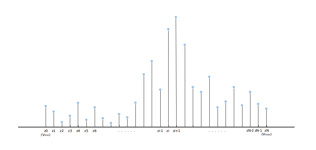

Where $z_i - z_{i-1} = \Delta z = (V_{min} - V_{max}) / N$, we assume that the range of the return $z_i$ is from $V_{min}$ to $V_{max}$, $N$ is the number of atoms, $(z_i, p_i(s, a))$. Now, for each state-action pair $(s, a)$, there is a corresponding distribution of its returns, not a expection value. We calculate the action value of $(s, a)$ as $Q(s, a) = E[Z(s, a)]$. Even through we still use the expected value, what we’re going to optimize is the distribution:

$\sup_{s, a} dist(R(s, a) + \gamma Z_{\bar{\theta}}(s', a^*), Z_{\theta}(s, a)) \\ a^* = \arg\max_{a′}Q(s′, a′) = \arg\max_{a′}E[Z(s′, a′)]$

The difference is obverse that, we still use a deep neural network to do function approximation, in traditional DQN, our output for each input state $s$ is a $|A|$-dim vector, each element corresponds to an action value $q(s, a)$, but now, the output for each input state $s$ is a $|A|*N$-dim matrix, that each row is a $N$-dim vector represents the return distribution of $Z(s, a)$, then we calculate the action-value of $(s, a)$ through:

$q(s, a) = E[Z(s, a)] = \sum\limits_{i=0}^{N} p_i(s, a) z_i$

KL Divergence
Now, we need to minimize the distance between the current distribution and the target distribution.
Note: the following content are mainly from that great blog: https://mtomassoli.github.io/2017/12/08/distributional_rl/#kl-divergence
If $p$ and $q$ are two distributions with same support (i.e. their $pdfs$ are non-zero at the same points), then their KL divergence is defined as follows:

$KL(p||q) = \int p(x) \log \frac{p(x)}{q(x)}dx \\ KL(p||q) = \sum\limits_{i=1}^{N} p(x_i) \log\frac{p(x_i)}{q(x_i)} = \sum\limits_{i=1}^{N} p(x_i)[ \log{p(x_i)} - \log{q(x_i)}]$

“Now say we’re using DQN and extract $(s, a, r, s′)$ from the replay buffer. A “sample of the target distribution” is $r + \gamma Z_{\bar{\theta}}(s′, a^*)$. We want to move $Z_{\theta}(s, a)$ towards this target (by keeping the target fixed).”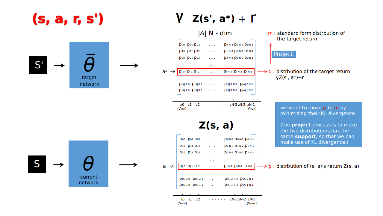

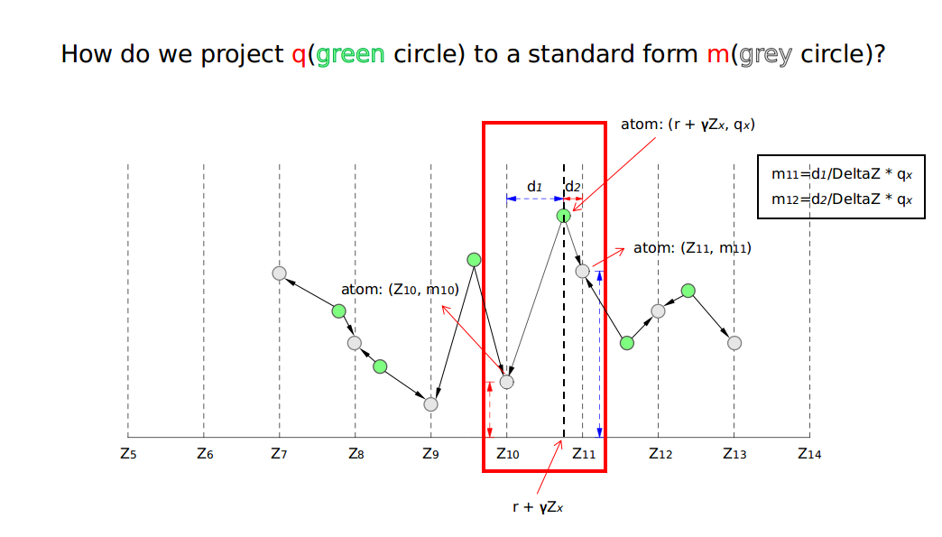
Then, their KL loss is:

$KL(m||p_{\theta}) = \sum\limits_{i=1}^{N} m_i \log\frac{m_i}{p_{\theta, i}} = \sum\limits_{i=1}^{N} m_i[ \log{m_i} - \log{p_{\theta, i}}] = H(m, p_{\theta}) − H(m)$

The gradient of the KL loss is:

$\nabla_{\theta} KL(m||p_{\theta}) = \nabla_{\theta} \sum\limits_{i=1}^{N} m_i \log\frac{m_i}{p_{\theta, i}} = \nabla_{\theta}[H(m, p_{\theta}) − H(m)] = \nabla_{\theta}H(m, p_{\theta})$

So, we can just use the cross-entropy:

$H(m, p_{\theta}) = - \sum\limits_{i=1}^{N} m_i \log{p_i(s, a; \theta)}$

as the loss function.

The total algorithm is as follows:

Do Distributional RL Based on Multi-Step Dueling Double DQN with Prioritized Experience Replay from scratch(basic version)
I feel really sorry to say that actually, this is a failed implementation, just as a reference, but I still hope it to be helpful to someone, and I promise I will try my best to fix it. Further more, I really hope some good guy can check my code, find the wrong place, even as a contributor to make it work together, thanks a lot.

8>Noisy DQN

Noisy DQN. Use stochastic network layers for exploration.
By now, the exploration method we used are all e-greedy methods, but in some games such as Montezuma’s Revenge, where many actions must be executed to collect the first reward. the limitations of exploring using ?-greedy policies are clear. Noisy Nets propose a noisy linear layer that combines a deterministic and noisy stream.
A normal linear layer with $p$ inputs and $q$ outputs, represented by:

$y = wx + b$

A noisy linear layer now is:

$y = (\mu^w + \sigma^w \odot \epsilon^w)x + (\mu^b + \sigma^b \odot \epsilon^b)$

Where where $\mu^w + \sigma^w \odot \epsilon^w$ and $\mu^b + \sigma^b \odot \epsilon^b$ replace $w$ and $b$, respectively. The parameters $\mu^w \in R^{q \times p}$, $\mu^b \in R^q$, $\sigma^w \in R^{q\times p}$ and $\sigma^b \in R^q$ are learnable whereas $\epsilon^w \in R^{q\times p}$ and $\epsilon^b \in R^q$ are noise random variables. There are two kinds of Gaussian Noise:

Independent Gaussian Noise:
The noise applied to each weight and bias is independent, where each entry $\epsilon^w_{i,j}$ (respectively each entry $\epsilon^b_j$) of the random matrix $\epsilon^w$ (respectively of the random vector $\epsilon^b$ ) is drawn from a unit Gaussian distribution. This means that for each noisy linear layer, there are $pq + q$ noise variables (for p inputs to the layer and q outputs).
Factorised Gaussian Noise:
By factorising $\epsilon^w_{i,j}$, we can use $p$ unit Gaussian variables $\epsilon_i$ for noise of the inputs and and $q$ unit Gaussian variables $\epsilon_j$ for noise of the outputs (thus $p + q$ unit Gaussian variables in total). Each $\epsilon^w_{i,j}$ and $\epsilon^b_j$ can then be written as:
$\epsilon^w_{i,j} = f(\epsilon_i)f(\epsilon_j) \\ \epsilon^b_j = f(\epsilon_j)$
where $f$ is a real-valued function. In our experiments we used $f(x) = sgn(x) \sqrt{|x|}$. Note that
for the bias $\epsilon^b_j$ we could have set $f(x) = x$, but we decided to keep the same output noise for weights and biases.

The total algorithm is as follows:

Do Noisy Network Based on Multi-Step Dueling Double DQN with Prioritized Experience Replay from scratch(basic version)

9>Rainbow

Finally, we get the integrated agent: Rainbow. It used a multi-step distributional loss:

$D_{KL}(\Phi_z d_t^{(n)} || d_t)$

Where $\Phi_z$ is the projection onto $z$, and the target distribution $d_t^{(n)}$ is:

$d_t^{(n)} =(R_t^{(n)} + \gamma_t^{(n)} z, p_\bar{\theta} (S_{t+n}, a^*_{t+n}))$

Using double Q-learning gets the greedy action $a^*_{t+n}$ of $S_{t+n}$ through online network, and evaluates such action using the target network.

In Rainbow, it uses the KL loss to prioritize transitions instead of using the absolute TD error, maybe more robust to noisy stochastic environments because the loss can continue to decrease even when the returns are not deterministic.

$p_t \propto (D_{KL}(\Phi_z d_t^{(n)} || d_t))^w$

The network architecture is a dueling network architecture adapted for use with return distributions. The network has a shared representation $f_{\xi}(s)$, which is then fed into a value stream $v_{\eta}$ with $N_{atoms}$ outputs, and into an advantage stream $a_{\xi}$ with $N_{atoms} \times N_{actions}$ outputs, where $a_{\xi}^i(f_{\xi}(s),a)$ will denote the output corresponding to atom $i$ and action $a$. For each atom $z^i$, the value and advantage streams are aggregated, as in dueling DQN, and then passed through a softmax layer to obtain the normalised parametric distributions used to estimate the returns’ distributions:

$p_{\theta}^i(s, a) = \frac{exp(v_{\eta}^i + a_{\Phi}^i(\phi, a) - \bar{a}_{\Phi}^i(s))}{\sum_j exp(v_{\eta}^j + a_{\Phi}^j(\phi, a) - \bar{a}_{\Phi}^j(s))}$

where $\phi = f_{\xi}(s)$, and $\bar{a}_{\Phi}^i(s) = \frac{1}{N_{actions}}\sum_{a’}a_{\Phi}^i(\phi, a’)$

Then replace all linear layers with their noisy equivalent(factorised Gaussian noise version).

Done, and thanks for reading, I hope it could be helpful to someone.
Any suggestion is more than welcome, thanks again.