RL_Paper_03

Rainbow: Combining Improvements in Deep Reinforcement Learning

Paper Source
Journal: The Thirty-Second AAAI Conference on Artificial Intelligence (AAAI-18)
Year: 2017
Institute: DeepMind
Author: Matteo Hessel, Joseph Modayil, Hado van Hasselt
#Deep Reinforcement Learning

Abstract

This paper examines six main extensions to DQN algorithm and empirically studies their combination. (It is a good paper which gives you a summary of several important technologies to alleviate the problems remaining in DQN and provides you some valuable insights in this research region.)
Baseline: Deep Q-Network(DQN) Algorithm Implementation in CS234 Assignment 2

1.INTRODUCTION
Because the traditional tabular methods are not applicable in arbitrarily large state spaces, we turn to those approximate solution methods (linear approximator & nonlinear approximator value-function approximation & policy approximation), which is to find a good approximate solution using limited computational resources. We can use a linear function, or multi-layer artificial neural networks, or decision tree as a parameterized function to approximate the value-function or policy.(More, see Sutton’s book Reinforcement Learning: An Introduction Chapter 9).
The following methods are all value-function approximation and gradient-based(using the gradients to update the parameters), and they all use experience replay and target network to eliminate the correlations present in the sequence of observations.
1> Linear
Using a linear function to approximate the value function(always the action value).

$\hat v(s, w) \doteq w^Tx(s) \doteq \sum \limits_{i=1}^d w_i x_i$

$w$ is the parameters, $x(s)$ is called a feature vector representing state $s$, and the state $s$ is the images(frames) observed by the agent in most time. So a linear approximator implemented with tensorflow can be just a fully-connected layer.

import tensorflow as tf
# state: a sequence of image(frame)
inputs = tf.layers.flatten(state)
# scope, which is used to distinguish q_params and target_q_params
out = layers.fully_connected(inputs, num_actions, scope=scope, reuse=reuse)

2> Nonlinear - DQN
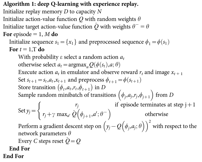
Deep Q-Network. The main difference of DQN from linear approximator is the architecture of getting the q_value, it is nonlinear.

And the total algorithm is as follows:

The approximator of DeepMind DQN implemented with tensorflow as described in their Nature paper can be:

import tensorflow as tf
with tf.variable_scope(scope, reuse=reuse) as _:
	conv1 = layers.conv2d(state, num_outputs=32, kernel_size=(8, 8), stride=4, activation_fn=tf.nn.relu)
	conv2 = layers.conv2d(conv1, num_outputs=64, kernel_size=(4, 4), stride=2, activation_fn=tf.nn.relu)
	conv3 = layers.conv2d(conv2, num_outputs=64, kernel_size=(3, 3), stride=1, activation_fn=tf.nn.relu)
	full_inputs = layers.flatten(conv3)
	full_layer = layers.fully_connected(full_inputs, num_outputs=512, activation_fn=tf.nn.relu)
	out = layers.fully_connected(full_layer, num_outputs=num_actions)

Do DQN from scratch(sample version)

3> Nonlinear - DDQN
Double DQN. The main difference of DDQN from DQN is the way of calculating the target q value.
As a reminder,
In Q-Learning:

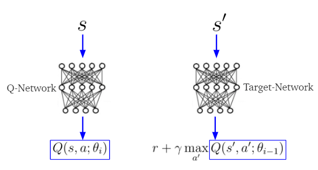
$Q(s,a) \leftarrow Q(s,a) + \alpha[r + \lambda max_{a'}Q(s',a') − Q(s,a)]$ $Y_t^{Q} = R_{t+1} + \lambda max_{a'}Q(S_{t+1},a') = R_{t+1} + \lambda Q(S_{t+1},argmax_{a'}Q(S_{t+1},a'))$

In DQN:

where $\theta_{i-1}$ is the target network parameters which is always represeted with $\theta_t^-$.

$Y_t^{DQN} = R_{t+1} + \lambda max_{a'}Q(S_{t+1},a';\theta_t^-)$

There is a problem with deep q-learning that “It is known to sometimes learn unrealistically high action values because it includes a maximization step over estimated action values, which tends to prefer overestimated to underestimated values” as said in DDQN paper.
The idea of Double Q-learning is to reduce overestimations by decomposing the max operation in the target into action selection and action evaluation.

$Y_t^{DoubleQ} = R_{t+1} + \lambda Q(S_{t+1}, argmax_{a'}Q(S_{t+1},a';\theta_t);\theta_t^-)$

Implement with tensorflow (the minimal possible change to DQN in cs234 assignment 2)

# DQN
q_samp = tf.where(self.done_mask, self.r, self.r + self.config.gamma * tf.reduce_max(target_q, axis=1))
actions = tf.one_hot(self.a, num_actions)
q = tf.reduce_sum(tf.multiply(q, actions), axis=1)
self.loss = tf.reduce_mean(tf.squared_difference(q_samp, q))

# DDQN
max_q_idxes = tf.argmax(q, axis=1)
max_actions = tf.one_hot(max_q_idxes, num_actions)
q_samp = tf.where(self.done_mask, self.r, self.r + self.config.gamma * tf.reduce_sum(tf.multiply(target_q, max_actions), axis=1))
actions = tf.one_hot(self.a, num_actions)
q = tf.reduce_sum(tf.multiply(q, actions), axis=1)
self.loss = tf.reduce_mean(tf.squared_difference(q_samp, q))

Do Double DQN from scratch(sample version)

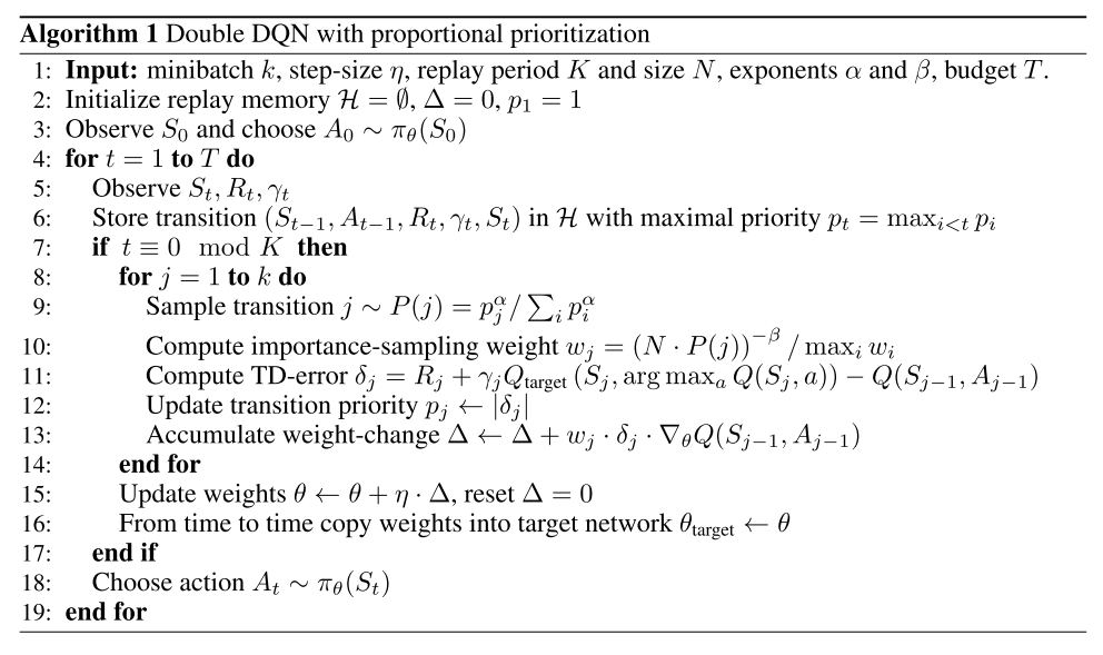
4>Prioritized experience replay
Prioritized experience replay. Improve data efficiency, by replaying more often transitions from which there is more to learn.
And the total algorithm is as follows:

Temporal-Difference(TD) Error
TD-Error: $r + \lambda V(s') - V(s)$
Where the value $r + \lambda V(s’) $ is known as the TD target.
Experiences with high magnitude TD error also appear to be replayed more often.
Stochastic Prioritization

Importance Sampling(IS)

5>Dueling network architecture
Dueling network architecture. Generalize across actions by separately representing state values and action advantages.

6>Multi-step bootstrap targets in A3C
Multi-step bootstrap targets. Shift the bias-variance tradeoff and helps to propagate newly observed rewards faster to earlier visited states.

7>Distributional Q-learning
Distributional Q-learning. Learn a categorical distribution of discounted returns, instead of estimating the mean.

8>Noisy DQN
Noisy DQN. Use stochastic network layers for exploration.

REFERENCES
1.Self Learning AI-Agents III:Deep (Double) Q-Learning(Blog)
2.【强化学习】Deep Q Network(DQN)算法详解(Bolg)